Four algorithms in one tiny brain

In the previous note I trained a small model on modular division. It built a Lissajous knot out of its output projection, and that knot was the algorithm.

This time I trained the same architecture on four tasks at once: division, addition, max, and parity. All four had to share one 4.8 M-parameter body and one output head. I ran five seeds at P = 149, WD = 0.3.

Every seed grokked all four tasks to at least 98% accuracy. Each task settled into its own shape, in its own basis, at its own time during training.

The four blooms

Below is one seed snapshotted every 200 steps, with one panel per task. Each panel shows that task's per-class L2 residual projected onto the top two principal directions of its own privileged basis: dlog Fourier for div, natural Fourier for add, top SVD for max, Nyquist axis for parity. Drag the slider to scrub through training.

The four tasks crystallise at very different times.

max comes online almost immediately, around step 250. There is barely anything to learn: the answer is just a or b, and the model uses copy-attention to point at whichever is larger.

parity, the bit (a+b) mod 2, groks around step 2,800. It needs exactly one Fourier mode, the Nyquist frequency k=74 on this 149-tooth clock. Once that one direction lines up, parity is done.

div takes longer, around step 4,200. It needs the discrete-logarithm Fourier basis, the same one I used in the previous note. Many frequencies have to cooperate.

add is the slowest, around step 5,300. Even though addition feels simpler than division to a human, it is the model's hardest task here. The reason was something I did not expect: add and parity share the Nyquist Fourier direction. While parity sits at the 50% "always guess the same bit" attractor, that direction is unavailable to add. Once parity finally pulls its two answer points apart along Nyquist, add can use the same direction to build the rest of its ring. The two grok timings move together within a few hundred steps of each other in every seed I ran.

Each algorithm needs its own glasses

This is the same final model, with each task's residuals projected into each task's basis. On the diagonal: each task in its own basis. Off the diagonal: the same task viewed through the wrong basis.

Div's ring only exists if you re-index the 148 invertible remainders by their discrete logarithm. In natural number order, the same 148 points look random.

Add's ring is the opposite: clean in natural order, noise in dlog. Max has no Fourier basis at all. It lives along a value-monotonic curve that is invisible to a Fourier projection in either order.

The short version: there is no universal coordinate system inside the model. Each algorithm picks its own, and looking through the wrong one turns geometry into static.

Where do the algorithms live?

The residual stream passes through nine recognisable points along the forward pass: the two input token embeddings (positions a and b), the input to block 0 (L0), the output of block 0's attention (attn0_out), the middle of FFN 0 (ffn0_mid), the input to block 1 (L1), the same two checkpoints inside block 1, and the final residual (L2). The grid below shows, per task, what the residual at each of those points looks like when projected onto its own top-2 PCs.

add's ring is already present in the token embedding for b. The model does not assemble add during forward, it bakes it into the input embeddings.

div's dlog ring first appears at attn0_out. Block 0's attention is where the discrete-logarithm transformation happens. Before that point div is noise. After it, div is a clean ring everywhere.

max's value-monotonic structure is present at every layer including the bare token embeddings. Copy-attention does not need to build geometry, the answer is just one of the inputs.

parity is two points on a single Nyquist axis, present from the start and progressively pulled apart by training.

Each algorithm has a different location signature.

Rebuilding the algorithms by hand

Once I knew how each of the four worked, the next thing to check was whether I could write them from scratch.

Three of the four are trivial.

div is the centrepiece of the previous note: a 2-block transformer with weights placed directly from the dlog-Fourier algorithm — no training — gets 100.00% on every (a, b) pair. W_E carries the dlog Fourier of the token id, attention copies it to the answer position, FFN1 computes single-frequency products via the SiLU linearisation trick, and W_U reads them back out.

add is the same construction with natural Fourier in place of dlog. Same machinery, simpler basis. I did not bother to write it out separately.

parity is rank-1. One Nyquist direction in W_U with sign (-1)^c, one bit out. A handful of lines of code.

max is the only one of the four that needed a genuinely different mechanism. It is not Fourier and not algebraic. The mechanism is copy-attention: Q·K monotonic in scalar value picks the position of the larger token, V copies that token's additive Fourier coefficients to the answer slot, and the head decodes via a Dirichlet kernel. So I built max by hand on a 4-head 2-block architecture matching the trained model.

The construction is visible directly in the token embeddings. Each value token v ∈ {0, …, 96} sits at exactly (cos k·v, sin k·v) on a circle of frequency k, in a pair of dimensions allocated to that mode. The non-value tokens (op, eq) carry zero in those dimensions and sit at the centre, off the circle.

Token embeddings at six different frequencies. The 97 value tokens lie on a clean circle by construction; op and eq sit at the centre.

After block 0's attention has picked the larger of a and b and copied that token's coefficients into the answer position, the residual at = carries the cos Fourier signature of max(a, b) exactly. The chart below puts the observed coefficients in blue against the closed-form prediction in red. They match.

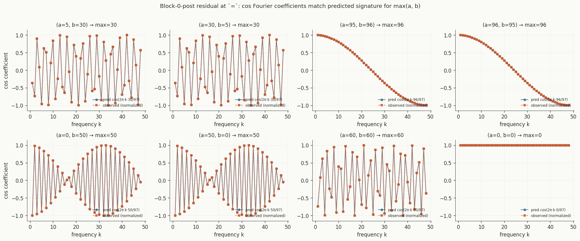
Post-block-0 residual at the = position. Each small panel is one (a, b) pair. Predicted cos Fourier coefficients of max(a, b) in red, observed in blue.

This is the strongest claim mechanistic interpretability can make on any given mechanism: not a description of what the model does, but a model built from understanding alone that does the same thing.

Driving the algorithms

Once the geometry is known, the model becomes controllable from outside. I tested four interventions, on all four tasks. For each: take the trained model, pick an input (a, b) it predicts correctly, capture its residual at L2, modify the residual, run the head, see what the model now predicts.

Chord walk shifts the residual by the vector between two manifold positions: h + (M[step(c, Δ)] − M[c]). Works for arbitrary Δ. Accuracy stays 97-100% across all four tasks for Δ from -100 to +100.

Linear tangent uses a single local tangent vector and scales it by Δ. Fails almost immediately for the non-trivial tasks. The algorithm curve has curvature, and a single tangent flies off it within one step.

Random shifts by a random vector of the same magnitude as the chord. Accuracy at chance, ~1/P.

Dictation replaces the residual with the precomputed answer-centroid for the desired class. 100% on all four tasks. This is a sanity check that the head reads the answer linearly from L2.

Two of the four interventions work at every shift on every task. That is more than a description of the algorithm. It is a working set of geometric levers on the model.

Multiple seeds

Same architecture, same data, five different random initial seeds. Each network grokked all four algorithms in a clean version of its own shape: a ring for div, a ring for add, a value cloud for max, two points on the Nyquist axis for parity. But the precise orientations of those shapes in 384-dimensional space differ between seeds.

The geometry is reproducible up to a gauge; the gauge itself is not. What is invariant across seeds is the type of object each task produces, not its frame. Part 3 will come back to this.

Where this leaves things

A multi-task model is not one geometric object, it is several. They share one residual stream, one set of weights, one forward pass. They emerge at different times during training. They live in different bases. They occupy different parts of the network. They can be coupled, as parity and add are through the Nyquist direction, or independent, as div and max are.

Knowing the geometry of one algorithm makes that mechanism auditable. Knowing the geometry of all of them makes the model auditable as a system.

Everything in this note happens on a small model on clean algebraic tasks, where the right basis is known from number theory. The next question is whether the same geometric picture survives in real LLMs — and, more importantly, whether the internal manifold can be turned into a supervision signal for the model's own training. That is Part 4.